12-23-2024
The goal here was to compare gene counts between rnaseq runs using
- The NCBI reference genome and gene annotations from the period of Roberto’s study (herein referred to as
NCBI Crassostrea gigas Annotation Release 101) - The most recent reference genome and gene annotations (herein referred to as
GCF_963853765.1-RS_2024_06) for C. gigas.
Motivation
As previously noted, in attemping to compare gene counts between
Roberto’s results and rnaseq results, we encountered the following hurdle:
The gene count matrix that Roberto provided predominantly used gene IDs prefixed with MSTRG_ (novel or unannotated genes/transcripts identified by
StringTie) and CGI_ (CpG islands), whereas the available NCBI annotations, and thus gene count data, for GCF_963853765.1-RS_2024_06 uses gene IDs prefixed with LOC_,
commonly used for annotated or predicted genes that don’t yet have an official gene symbol or name.
However, we found that the NCBI Crassostrea gigas Annotation Release 101 NCBI genome and annotations did use LOC_ gene IDs, which facilitates matching by ID
rather than requiring BLAST or other indirect gene ID matching methods.
So, for this current task, we used the NCBI Crassostrea gigas Annotation Release 101
reference genome (linked above) as as a proxy for Roberto’s, supported by the fact that it represents the state of the art at the time of his publication.
Because we’re only varying the reference genome and annotations here, keeping the derivation of gene counts via rnaseq fixed, this task is primaraily an exploration of the effect of using the updated reference genome and annotations during reanalysis. This may provide insight when doing future reanalysis where the reference genome and annotations have been updated since an original study.
Secondarily, we may wish to see whether Principal Component Analysis reveals significant contributions from the genes that Roberto cites.
Method
We ran rnaseq on Seqera usnig NCBI Crassostrea gigas Annotation Release 101 using the following parameters, which are identical to the GCF_963853765.1-RS_2024_06 run with the obvious exceptions of reference genome and annotation paths:
{
    "remove_ribo_rna": false,
    "help_full": false,
    "custom_config_base": "https://raw.githubusercontent.com/nf-core/configs/master",
    "skip_deseq2_qc": false,
    "gencode": false,
    "umitools_dedup_stats": false,
    "plaintext_email": false,
    "save_reference": false,
    "skip_markduplicates": false,
    "ribo_database_manifest": "/.nextflow/assets/nf-core/rnaseq/workflows/rnaseq/assets/rrna-db-defaults.txt",
    "monochrome_logs": false,
    "aligner": "star_salmon",
    "featurecounts_group_type": "gene_biotype",
    "save_bbsplit_reads": false,
    "skip_multiqc": false,
    "skip_preseq": true,
    "skip_dupradar": false,
    "save_align_intermeds": false,
    "gtf": "https://steveyost-seqera.s3.us-east-1.amazonaws.com/Cgigas_ArredondoEspinoza2023/run_ncbi_dataset_GCA_000297895.1_GCF/genomic_removed_empty_gene_ids.gtf",
    "max_multiqc_email_size": "25.MB",
    "save_trimmed": false,
    "bracken_precision": "S",
    "min_trimmed_reads": 10000,
    "skip_fastqc": false,
    "pseudo_aligner_kmer_size": 31,
    "deseq2_vst": true,
    "umitools_extract_method": "string",
    "validate_params": true,
    "bam_csi_index": false,
    "extra_fastp_args": "--cut_mean_quality 30 --trim_front1 10 --trim_front2 10",
    "with_umi": false,
    "skip_qc": false,
    "version": false,
    "trimmer": "fastp",
    "publish_dir_mode": "copy",
    "input": "s3://steveyost-seqera/Cgigas_ArredondoEspinoza2023/fetchngs/samplesheet/samplesheet_for_rnaseq.csv",
    "skip_bigwig": false,
    "igenomes_base": "s3://ngi-igenomes/igenomes/",
    "skip_gtf_transcript_filter": false,
    "stringtie_ignore_gtf": false,
    "skip_umi_extract": false,
    "kallisto_quant_fraglen_sd": 200,
    "save_unaligned": false,
    "featurecounts_feature_type": "exon",
    "multiqc_title": "rnaseq_Cgigas_ArredondoEspinoza2023",
    "skip_gtf_filter": false,
    "custom_config_version": "master",
    "fasta": "https://steveyost-seqera.s3.us-east-1.amazonaws.com/Cgigas_ArredondoEspinoza2023/run_ncbi_dataset_GCA_000297895.1_GCF/GCF_000297895.1_oyster_v9_genomic.fna",
    "hisat2_build_memory": "200.GB",
    "skip_rseqc": false,
    "save_non_ribo_reads": false,
    "save_kraken_unassigned": false,
    "skip_alignment": false,
    "skip_qualimap": false,
    "star_ignore_sjdbgtf": false,
    "skip_stringtie": false,
    "gtf_extra_attributes": "gene_name",
    "save_merged_fastq": false,
    "save_umi_intermeds": false,
    "save_kraken_assignments": false,
    "show_hidden": false,
    "min_mapped_reads": 5,
    "rseqc_modules": "bam_stat,inner_distance,infer_experiment,junction_annotation,junction_saturation,read_distribution,read_duplication",
    "gtf_group_features": "gene_id",
    "skip_trimming": false,
    "kallisto_quant_fraglen": 200,
    "igenomes_ignore": false,
    "skip_pseudo_alignment": true,
    "outdir": "s3://steveyost-seqera/Cgigas_ArredondoEspinoza2023/run_ncbi_dataset_GCA_000297895.1_GCF/",
    "skip_bbsplit": true,
    "pipelines_testdata_base_path": "https://raw.githubusercontent.com/nf-core/test-datasets/7f1614baeb0ddf66e60be78c3d9fa55440465ac8/",
    "help": false,
    "stranded_threshold": 0.8,
    "unstranded_threshold": 0.1,
    "umitools_grouping_method": "directional",
    "skip_biotype_qc": false
}
With the resulting salmon.merged.gene_counts.tsv files from each run in hand, I then queried ChatGPT 4o for recommendations on visually comparing gene counts. Its recommendations included a Venn diagram to indicate matching/non-matching gene IDs and scatter plots showing gene counts on X and Y axes for matching gene IDs for the respective runs.
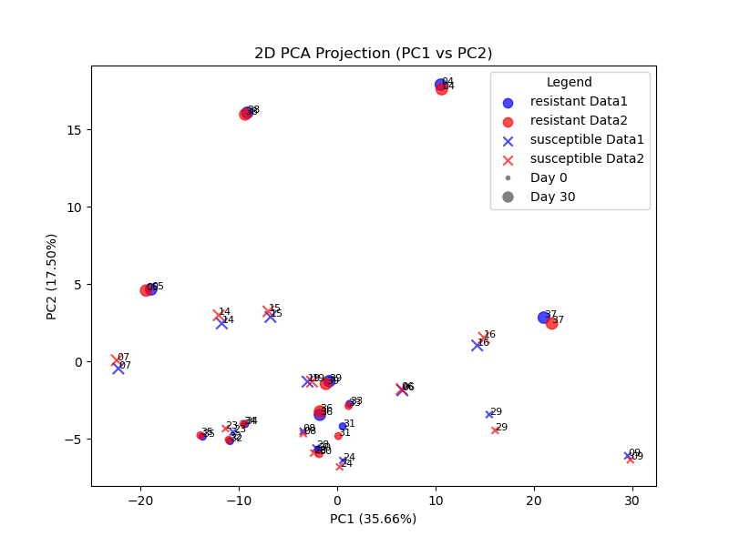
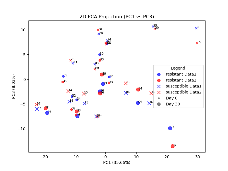
Further, to visualize the gene count differences between the rnaseq runs using the NCBI Crassostrea gigas Annotation Release 101 and GCF_963853765.1-RS_2024_06 reference genomes and annotations, I chose PCA among the recommendations made by ChatGPT 4o, and interactively worked with it to produce a 2D PCA plot which, with additional metadata for the samples, differentiates the two runs (by color), and each sample’s noted resilience, and time interval (day 0 vs. day 30). Satisfied with this, and noting the striking similarity between the two runs, I then had ChatGPT produce an interactive 3D PCA plot to see whether greater differences appeared given a third principal component axis. Figures below show the PC1/PC2 and PC1/PC3 planar projections, and an interactive 3D plot is shown.
Results


Possible further work
For each PCA component, examine the PCA loadings.
Identify which genes contribute most to the separation, and examine correlation of those genes with changes noted in annotation comparisons between GCF_963853765.1-RS_2024_06 and NCBI Crassostrea gigas Annotation Release 102 (found here ) and then between NCBI Crassostrea gigas Annotation Release 102 and NCBI Crassostrea gigas Annotation Release 101 (found here ).
See also the Comparison of the current and previous annotations section of the GCF_963853765.1-RS_2024_06 Annotation Report and the same section of the Roslin Annotation Report
Our hypothesis would be that genes contributing to Data1-Data2 separation would be the ones with poor mappings (e.g. major changes) between reference genomes. Determine if these genes are disproportionately affected by the differences in reference genomes.
Code
Below is the python script that generated the above Venn diagram and scatter plots:
import pandas as pd
import matplotlib.pyplot as plt
from matplotlib_venn import venn2
import matplotlib
import numpy as np

# Use non-interactive backend for headless environments
matplotlib.use('Agg')

# Function to load gene count files (ignoring the second column)
def load_gene_counts(file_path):
    df = pd.read_csv(file_path, sep='\t')
    df = df.drop(columns=df.columns[1])  # Drop the second column (gene_name)
    return df

# Function to prepare the comparison table
def compare_gene_counts(df1, df2):
    # Merge data on gene_id
    # The suffixes modifies the column names for the respective dataframes
    merged = pd.merge(df1, df2, on='gene_id', how='outer', suffixes=('_run1', '_run2'))

    # Mark presence in each run
    # : is the row indexer; it means select all rows
    # 1 selects the second column
    # len(df1.columns selects the first column in df2 data
    # The 'present_in' columns are appended to each row
    # Only one column of each original dataframe is checked because the outer
    # join assigns NaN to all colums if the joined-on key isn't present.
    merged['present_in_run1'] = ~merged.iloc[:, 1].isna()
    merged['present_in_run2'] = ~merged.iloc[:, len(df1.columns)].isna()

    return merged

# Function to generate visualizations
def generate_visualizations(merged_df, output_prefix, df1_columns):
    # Venn Diagram
    only_in_run1 = merged_df['present_in_run1'] & ~merged_df['present_in_run2']
    only_in_run2 = merged_df['present_in_run2'] & ~merged_df['present_in_run1']
    in_both_runs = merged_df['present_in_run1'] & merged_df['present_in_run2']

    venn2(
        subsets=(only_in_run1.sum(), only_in_run2.sum(), in_both_runs.sum()),
        set_labels=('Run 1', 'Run 2')
    )
    plt.title("Gene ID Overlap Between Runs")
    plt.savefig(f"{output_prefix}_venn.png")
    plt.clf()

    # Scatter Plot for common genes
    common_genes = merged_df[merged_df['present_in_run1'] & merged_df['present_in_run2']]

    plt.xlabel("Log2 Run 1 Counts")
    plt.ylabel("Log2 Run 2 Counts")
    plt.title(f"Scatter Plot of Log2 Gene Counts for Common Genes")
    plt.grid(True)
    for col_idx in range(1, len(df1_columns)):
        column_name = df1_columns[col_idx]
        print(f"Processing sample: {column_name}")
        sample_1_run1 = column_name + '_run1'
        sample_1_run2 = column_name + '_run2'

        # Check if columns exist before plotting
        if sample_1_run1 in common_genes.columns and sample_1_run2 in common_genes.columns:
            x = np.log2(common_genes[sample_1_run1] + 1)
            y = np.log2(common_genes[sample_1_run2] + 1)

            plt.scatter(x, y, alpha=0.3, s=5)  # Reduced dot size (s=5)
        else:
            print(f"Error: Columns {sample_1_run1} or {sample_1_run2} not found in the merged dataset.")
    plt.savefig(f"{output_prefix}_scatter.png")

# Main Function
def main(file1, file2, output_prefix):
    # Load data
    df1 = load_gene_counts(file1)
    df2 = load_gene_counts(file2)

    # Perform comparison
    merged_df = compare_gene_counts(df1, df2)

    # Save tabular comparison
    merged_df.to_csv(f"{output_prefix}_comparison.csv", index=False)

    # Generate visualizations
    generate_visualizations(merged_df, output_prefix, df1.columns)

# Example usage:
# main("run1_counts.tsv", "run2_counts.tsv", "gene_comparison")


# Example usage:
main("ncbi_dataset_GCA_000297895.1/ncbi_dataset/data/GCF_000297895.1/salmon.merged.gene_counts.tsv", "seqera_roberto/salmon.merged.gene_counts_seqera.tsv", "gene_comparison")
Below is the code for generating the 3D PCA plot, as generated by ChatGPT 4o and subsequently modified.
# Import required libraries
import pandas as pd
import numpy as np
from sklearn.decomposition import PCA
from sklearn.preprocessing import StandardScaler
import matplotlib
import matplotlib.pyplot as plt
from mpl_toolkits.mplot3d import Axes3D
import plotly.graph_objects as go

matplotlib.use('Agg')

destdir = '/mnt/c/Users/inter/Downloads/GMGI/ChatGPT/'
# Load the files
data1_file = f'{destdir}salmon.merged.gene_counts_2023_seqera.tsv'
data2_file = f'{destdir}salmon.merged.gene_counts_roberto_seqera.tsv'
metadata_file = f'{destdir}deseq_metadata2.csv'

# Load the data1 and data2, ignoring the second column
data1 = pd.read_csv(data1_file, sep='\t', index_col=0).iloc[:, 1:]
data2 = pd.read_csv(data2_file, sep='\t', index_col=0).iloc[:, 1:]

# Load the metadata
metadata = pd.read_csv(metadata_file)

# Find common genes between data1 and data2
common_genes = data1.index.intersection(data2.index)

# Subset both datasets to include only these common genes
data1_common = data1.loc[common_genes]
data2_common = data2.loc[common_genes]

# Compute variance for each gene in the common data
variances = data1_common.var(axis=1) + data2_common.var(axis=1)

# Select the top 500 most variable genes
top_genes = variances.nlargest(500).index
data1_top = data1_common.loc[top_genes]
data2_top = data2_common.loc[top_genes]

# Standardize the gene counts
scaler = StandardScaler()
data1_standardized = pd.DataFrame(
    scaler.fit_transform(data1_top.T).T, index=data1_top.index, columns=data1_top.columns
)
data2_standardized = pd.DataFrame(
    scaler.fit_transform(data2_top.T).T, index=data2_top.index, columns=data2_top.columns
)

# Perform PCA to reduce to 3 components
pca1 = PCA(n_components=3)
pca2 = PCA(n_components=3)
pca1_results = pd.DataFrame(
    pca1.fit_transform(data1_standardized.T),
    index=data1_standardized.columns,
    columns=["PC1", "PC2", "PC3"]
)
pca2_results = pd.DataFrame(
    pca2.fit_transform(data2_standardized.T),
    index=data2_standardized.columns,
    columns=["PC1", "PC2", "PC3"]
)

# Merge PCA results with metadata
metadata_subset = metadata.set_index("sample")
pca1_metadata = pca1_results.join(metadata_subset, how="inner")
pca2_metadata = pca2_results.join(metadata_subset, how="inner")

# Combine PCA results for both datasets
pca1_metadata['Dataset'] = 'Data1'
pca2_metadata['Dataset'] = 'Data2'
pca_combined = pd.concat([pca1_metadata, pca2_metadata], axis=0)

# Marker mapping
pca_combined['Marker'] = pca_combined['thermal.tolerance'].map(
    {'resistant': 'o', 'susceptible': 'x'}
)
# pca_combined['Marker Size'] = pca_combined['day'].map({0: 5, 30: 15})
pca_combined['Marker Size'] = pca_combined['day'].map({0: 3, 30: 8})


# Marker size adjustment is necessary for the 3D plot
def marker_size(row):
    if row['day'] == 30:
        return row['Marker Size'] * (1.5 if row['Marker'] == 'o' else 0.6)
    return row['Marker Size'] * (2.2 if row['Marker'] == 'o' else 1.4)


pca_combined['Scaled Marker Size'] = pca_combined.apply(
    lambda row: marker_size(row), axis=1
)

# Interactive 3D PCA plot with updated marker styles
fig = go.Figure()

# Add Data1 points with markers
data1_points = pca_combined[pca_combined['Dataset'] == 'Data1']
fig.add_trace(go.Scatter3d(
    x=data1_points['PC1'],
    y=data1_points['PC2'],
    z=data1_points['PC3'],
    mode='markers+text',
    marker=dict(
        size=data1_points['Scaled Marker Size'],
        color='blue',
        symbol=data1_points['Marker'].map({'o': 'circle', 'x': 'x'})
    ),
    name='Data1',
    text=data1_points.index.str[-2:],  # Sample ID as last two digits
    textposition='top center'
))

# Add Data2 points with markers
data2_points = pca_combined[pca_combined['Dataset'] == 'Data2']
fig.add_trace(go.Scatter3d(
    x=data2_points['PC1'],
    y=data2_points['PC2'],
    z=data2_points['PC3'],
    mode='markers+text',
    marker=dict(
        size=data2_points['Scaled Marker Size'],
        color='red',
        symbol=data2_points['Marker'].map({'o': 'circle', 'x': 'x'})
    ),
    name='Data2',
    text=data2_points.index.str[-2:],  # Sample ID as last two digits
    textposition='top center'
))

# Update layout
fig.update_layout(
    title="Interactive 3D PCA Plot",
    scene=dict(
        xaxis_title=f'PC1 ({pca1.explained_variance_ratio_[0]*100:.2f}%)',
        yaxis_title=f'PC2 ({pca1.explained_variance_ratio_[1]*100:.2f}%)',
        zaxis_title=f'PC3 ({pca1.explained_variance_ratio_[2]*100:.2f}%)',
    ),
    scene_camera=dict(
        up=dict(x=0, y=1, z=0),
        eye=dict(x=0, y=0, z=2.5)  # Adjust perspective to make PC1 horizontal and PC2 vertical
    ),
    legend=dict(title="Dataset")
)

# Save interactive 3D plot as HTML
html_path = f'{destdir}/Interactive_3D_PCA_Plot.html'
fig.write_html(html_path)


# Create static 2D PCA plots with markers
def plot_2d_pca(data, x, y, title, xlabel, ylabel, filename):
    fig, ax = plt.subplots(figsize=(8, 6))
    for (thermal_tolerance, marker), color in [
        (('resistant', 'o'), 'blue'), (('susceptible', 'x'), 'red')
    ]:
        subset = data[(data['thermal.tolerance'] == thermal_tolerance) & (data['Dataset'] == 'Data1')]
        ax.scatter(
            subset[x], subset[y], c='blue', alpha=0.7, label=f'{thermal_tolerance} Data1',
            marker=marker, s=subset['Marker Size'] * 10
        )
        for i, txt in enumerate(subset.index):
            ax.annotate(txt[-2:], (subset[x].iloc[i], subset[y].iloc[i]), fontsize=8)

        subset = data[(data['thermal.tolerance'] == thermal_tolerance) & (data['Dataset'] == 'Data2')]
        ax.scatter(
            subset[x], subset[y], c='red', alpha=0.7, label=f'{thermal_tolerance} Data2',
            marker=marker, s=subset['Marker Size'] * 10
        )
        for i, txt in enumerate(subset.index):
            ax.annotate(txt[-2:], (subset[x].iloc[i], subset[y].iloc[i]), fontsize=8)

    ax.set_xlabel(xlabel)
    ax.set_ylabel(ylabel)
    plt.title(title)
    handles, _labels = ax.get_legend_handles_labels()
    handles.extend([
        plt.Line2D([0], [0], marker='o', color='w', markerfacecolor='gray', markersize=6, label='Day 0'),
        plt.Line2D([0], [0], marker='o', color='w', markerfacecolor='gray', markersize=10, label='Day 30')
    ])
    ax.legend(handles=handles, title="Legend")
    plt.savefig(f'{destdir}{filename}.png')
    plt.close()

# Regenerate 2D PCA projections
plot_2d_pca(
    pca_combined, 'PC1', 'PC2',
    "2D PCA Projection (PC1 vs PC2)",
    f'PC1 ({pca1.explained_variance_ratio_[0]*100:.2f}%)',
    f'PC2 ({pca1.explained_variance_ratio_[1]*100:.2f}%)',
    "2D_PCA_PC1_PC2"
)
plot_2d_pca(
    pca_combined, 'PC1', 'PC3',
    "2D PCA Projection (PC1 vs PC3)",
    f'PC1 ({pca1.explained_variance_ratio_[0]*100:.2f}%)',
    f'PC3 ({pca1.explained_variance_ratio_[2]*100:.2f}%)',
    "2D_PCA_PC1_PC3"
)